6.11.1. Modeling climatic effects on insect distributions
The abundance of any poikilothermic species is determined largely by proximate ecological factors including the population densities of predators and competitors (section 13.4) and interactions with habitat, food availability, and climate. Although the distributions of insect species result from these ecological factors, there is also a historical component. Ecology determines whether a species can continue to live in an area; history determines whether it does, or ever had the chance to live there. This difference relates to timing; given enough time, an ecological factor becomes a historical factor. In the context of present-day studies of where invasive insects occur and what the limits of their spread might be, history may account for the original or native distribution of a pest. However, knowledge of ecology may allow prediction of potential or future distributions under changed environmental conditions (e.g. as a result of the “greenhouse effect”; see section 6.11.2) or as a result of accidental (or intentional) dispersal by humans. Thus, ecological know- ledge of insect pests and their natural enemies, especially information on how climate influences their development, is vital for the prediction of pest out- breaks and for successful pest management.
There are many models pertaining to the population biology of economic insects, especially those affecting major crop systems in western countries. One example of a climatic model of arthropod distribution and abundance is the computer-based system called CLIMEX (developed by R.W. Sutherst and G.F. Maywald), which allows the prediction of an insect’s potential relative abundance and distribution around the world, using ecophysiological data and the known geographical distribution. An annual “ecoclimatic index” (EI), describing the climatic favorability of a given location for permanent colonization of an insect species, is derived from a climatic database combined with estimates of the response of the organisms to temperature, moisture, and day length. The EI is calculated as follows (Fig. 6.14). First, a population growth index (GI) is determined from weekly values averaged over a year to obtain a measure of the potential for population increase of the species. The GI is estimated from data on the seasonal incidence and relative abundance in different parts of the species’ range. Second, the GI is reduced by incorporation of four stress indices, which are measures of the deleterious effects of cold, heat, dry, and wet.
Commonly, the existing geographical distribution and seasonal incidence of a pest species are known but biological data pertaining to climatic effects on development are scanty. Fortunately, the limiting effects of climate on a species usually can be estimated reliably from observations on the geographical distribution. The climatic tolerances of the species are inferred from the climate of the sites where the species is known to occur and are described by the stress indices of the CLIMEX model. The values of the stress indices are progressively adjusted until the CLIMEX predictions agree with the observed distribution of the species. Naturally, other information on the climatic tolerances of the species should be incorporated where possible because the above procedure assumes that the present distribution is climate limited, which might be an oversimplification.
Such climatic modeling based on world data has been carried out for tick species and for insects such as the Russian wheat aphid, the Colorado potato beetle, screw-worm flies, biting flies of Haematobia species, dung beetles, and fruit flies (Box 6.3). The output has great utility in applied entomology, namely in epidemiology, quarantine, management of insect pests, and entomological management of weeds and animal pests (including other insects).
In reality, detailed information on ecological performances may never be attained for many taxa, although such data are essential for the autecological-based distribution models described above. Nonetheless, there are demands for models of distribution in the absence of ecological performance data. Given these practical constraints, a class of modeling has been developed that accepts distribution point data as surrogates for “performance (process) characteristics” of organisms. These points are defined bioclimatically, and potential distributions can be modeled using some flexible procedures. Analyses assume that current species distributions are restricted (constrained) by bioclimatic factors. A suite of models developed in Australia (e.g. BIOCLIM, developed by Henry Nix and colleagues) allow estimation of potential constraints on species distribution in a stepwise process. First, the sites at which a species occurs are recorded and the climate estimated for each data point, using a set of bioclimatic measures based on the existing irregular network of weather stations across the region under consideration. Factors such as annual precipitation, seasonality of precipitation, precipitation of the driest quarter, minimum temperature of the coldest period, maximum temperature of the warmest period, and elevation appear to be particularly influential and are likely to have wide significance in determining the distribution of poikilothermic organisms. From this information a bioclimatic profile is developed from the pooled climate per site estimates, providing a profile of the range of climatic conditions at all sites for the species. Next, the bioclimatic profiles so produced are matched with climate estimates at other mapped sites across a regional grid to identify all other locations with similar climates. Specialized software then can be used to measure similarity of sites, with comparison being made via a digital elevation model with fine resolution. All locations within the grid with similar climates to the species-profile form a predicted bioclimatic domain. This is represented spatially (mapped) as a “predicted potential distribution” for the taxon under consideration, in which isobars (or colors) represent different degrees of confidence in the prediction of presence.
The estimated potential distribution of the chirono-mid midge genus Austrochlus (Diptera) based on data points in south-western Australia is shown in Fig. 6.15. Based on climatic (predominantly seasonal rainfall) parameters, dark locations show high probability of occurrence and light grey show less likelihood. The model, based on two well-surveyed, partially sympatric species from south-western Australia, predicts the occurrence of an ecologically related taxon in central Australia, which has been since discovered within the predicted range. The effectiveness of bioclimatic modeling in predicting distributions of sister taxa, as shown here and in other studies, implies that much speciation has been by vicariance, with little or no ecological divergence (section 8.6).
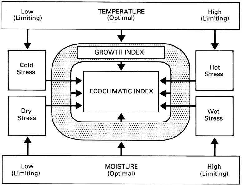
The EI value describes the climatic favorability of a given location for a given species. Comparison of EI values allows different locations to be assessed for their relative suitability to a particular species. (After Sutherst & Maywald 1985)
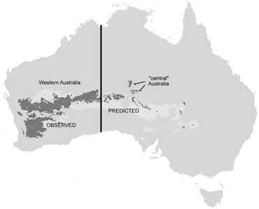
Black, predicted presence within 98% confidence limits; pale grey, within 95% confidence. (After Cranston et al. 2002)

